Linear Regression

To conduct linear regression, check the distribution of your variables as the linear regression works well with the normally distributed data. Try transforming your scale variables to make them normally distributed or close to normally distributed. To test the normality of your data follow these steps.

Testing Normality

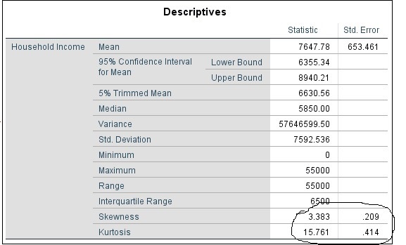
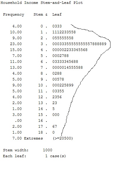
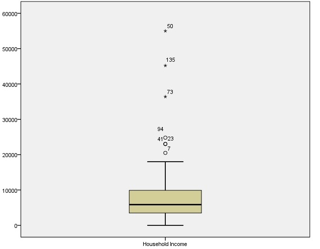
Analyze->Descriptive->Explore will give you test for normality of the desired variable. The scores of skewness, kurtosis and standard error are the key statistics to watch out. The ratio of kurtosis to standard error is greater than two, indicates deviation from normality. Further, stef-and-leaf plot shows the shape of normal curve of the variable. Box plot tells the cases that lies outside the normal range adding non-normality to your data. The figures illustrates these scores and plots for a sample household income data.

The image below with suggestive pencil sketch shows the line of an imaginary non-normal curve over the obtained data. This suggests the data is right-skewed with a right long tail.

Likewise the box-plot suggests the outlier cases.

Before, including income variable in my linear model, it will be good to transform it close to normality. This can be done either by dropping the outliers or transforming the variable. We will discuss in more detail in coming sub-sections.

Lets get back to the linear regression again.

These are the important statistics to select while doing Analyze->Regression->Linear

Estimates

The beta coefficients will be obtained for our reporting purpose.

Model fit

This assesses the model fit criteria by reporting the R-sqaure and other measures.

Part and partial correlations

The correlation scores of each independent predictor variable will give idea about robustness of our estimates.

Collinearity diagnostics

This will assess the collinearity problem between variables.

These are the scores to report from the output tables

Model summary

The key values from this table to report are- R square and adjusted R square. The R-square suggests how much percentage of variance in the outcome variable is explained the independent variables of this model. For example, if R square is 0.32, this means 32% of variance is explained. Hence, initially, high R-square value is a good sign. However, the adjusted R-square is more robust as it also accounts for the number of variables we include in the model. So, usually, adjusted R-square is less than R square value. Both the values help evaluating the model fit.

ANOVA

If ANOVA statistics (F-value) is significant in the ANOVA table, it indicates the model is better to use than simply guessing means of variables.

Coefficients table

From this table, report the unstandardized beta coefficients and associated standard errors. See the significance levels according to your own alpha standards (.00, 0.05, 0.01). If the coefficients are significants, the beta values are considered significant for that independent variable.

The other portion of this table assesses the multicollinearity. VIF is less than 2, then the model is in the acceptable limits of multicollinearity. tolerance is simply inverse of VIF. For reporting, VIF is used.

Collinearity diagnostic

If multiple eigen values are close to 0, and Condition index>15, this means collinearity problems.

Trouble with Linear Regression

Some commonly faced problems and treatment can be seen as follows.

Mutlicollinearity

High VIF scores (>2) followed by multiple negative Eigen values are poor fit. This can be handled by either or combination of these.

Treatment

Use z-scores and try replacing unimportant variables. You can simply replace the original values of the variables with their computed z-score in your model. To compute z-score, go Analyze->Descriptive statistics->Descriptive. Select the variable(s) that needs to be standardized, check the box below reading ‘save standardized values as variables’.

Removal of outliers

If the sample size is large and dropping a few outlier cases, doesn’t likely to affect the results, try deleting them and save the data file file with new name and re-run the regression. It is generally not a good option to loose the valuable data.

Transformation

Usually, transforming the variable is better option than to drop them. Some useful transformations are natural log (ln) and Log with base 10, square root, inverse etc. If the purpose is to not the predict the outcome data with accuracy, instead to have an idea of relationship between outcome and input variables (as in the most cases of social science research), it is always good to transform the variables.

Further treatment

If these don’t work, factor analysis and using factor scores in the regression can be tried.

For the purpose of basic to intermediate level analysis, the tutorial so far should be handy.